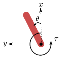
Controlled Pendulum

Open in molab

This example stabilizes the classical torque-driven pendulum benchmark. The plant state is angle \(\theta\) and angular velocity \(\omega\), and the control variable is pivot torque \(\tau\).

The example is intentionally small, but it exercises the main Regelum ideas: continuous dynamics are declared as a right-hand side, discrete nodes declare their state reads, and phases turn those local declarations into an executable schedule.

Dynamics

The plant uses the uniform-rod pendulum dynamics

\[ \dot{\theta} = \omega, \qquad \dot{\omega} = \frac{3g}{2\ell}\sin(\theta) + \frac{3\tau}{m\ell^2}. \]

The controller is a clipped PD law around the upright equilibrium:

\[ \tau = \operatorname{clip}_{[-\tau_{\max}, \tau_{\max}]} \left(-k_p\operatorname{atan2}(\sin\theta,\cos\theta)-k_d\omega\right). \]

The executable example uses \(g=9.81\), \(\ell=1.0\), \(m=1.0\), \(k_p=14.0\), \(k_d=4.0\), and \(\tau_{\max}=4.0\). The plant is integrated at 100 Hz with dt="0.01", while the controller runs at 20 Hz with dt="0.05". Between controller updates, Controller.State.tau is sampled and held.

Logical Nodes

The closed-loop model is decomposed into four logical nodes:

Node	Role
pendulum_plant	An ODESystem wrapping PendulumODE; it integrates \(\theta,\omega\) and reads held \(\tau\).
observer	Reads plant state and publishes sin_theta, cos_theta, and omega.
controller	Reads observer features and writes saturated tau.
logger	Reads plant state, clock time, and held torque, then appends a sample.

That split is the point of the example. The plant does not know how torque is computed. The controller does not know how the ODE is integrated. The logger does not own any of the physical state. Each node declares only the state it owns and the ports it reads.

Define The Plant

PendulumODE is the continuous primitive. It inherits from rg.ODENode, so it only specifies state and dstate(...); integration settings are supplied later by rg.ODESystem.

class PendulumODE(rg.ODENode):
    mass: float = 1.0
    length: float = 1.0
    gravity: float = 9.81

    def __init__(self, theta0: float, omega0: float) -> None:
        self.theta0 = theta0
        self.omega0 = omega0

    class State(rg.NodeState):
        theta: float = rg.var(init=lambda self: cast(PendulumODE, self).theta0)
        omega: float = rg.var(init=lambda self: cast(PendulumODE, self).omega0)

    def dstate(
        self,
        state: State,
        tau: float = rg.src(lambda: Controller.State.tau),
    ) -> State:
        tau_c = 3.0 / (self.mass * self.length**2)
        g_c = (3.0 * self.gravity) / (2.0 * self.length)
        return self.State(
            theta=state.omega,
            omega=g_c * ca.sin(state.theta) + tau_c * tau,
        )

The theta and omega variables use lazy initializers. At runtime the node instance is passed to the initializer, so the constructor values become the initial ODE state.

The torque input uses a lazy source reference: rg.src(lambda: Controller.State.tau). The lambda only delays evaluation until Controller exists in the Python module. Semantically it is still a plain state-port read.

Observer

Observer is an ordinary discrete node. This snippet uses a separate Inputs namespace, which is useful when a node has several named reads.

class Observer(rg.Node):
    class State(rg.NodeState):
        sin_theta: float
        cos_theta: float
        omega: float

    class Inputs(rg.NodeInputs):
        theta: float = rg.src(PendulumODE.State.theta)
        omega: float = rg.src(PendulumODE.State.omega)

    def update(self, inputs: Inputs) -> State:
        return self.State(
            sin_theta=math.sin(inputs.theta),
            cos_theta=math.cos(inputs.theta),
            omega=inputs.omega,
        )

The return value is a new Observer.State object. Regelum commits it after the node runs, and later nodes in the same phase can read those ports.

Controller

Controller shows the compact input style: inputs are declared directly in the update(...) signature. This is equivalent to a separate Inputs namespace.

class Controller(rg.Node):
    dt: str = "0.05"
    tau_max: float = 4.0

    def __init__(self, kp: float, kd: float) -> None:
        self.kp = kp
        self.kd = kd

    class State(rg.NodeState):
        tau: float

    def update(
        self,
        sin_theta: float = rg.src(Observer.State.sin_theta),
        cos_theta: float = rg.src(Observer.State.cos_theta),
        omega: float = rg.src(Observer.State.omega),
    ) -> State:
        theta = math.atan2(sin_theta, cos_theta)
        raw = -self.kp * theta - self.kd * omega
        tau = float(np.clip(raw, -self.tau_max, self.tau_max))
        return self.State(tau=tau)

The class-level dt means the controller runs every 0.05 seconds. The plant integrates every 0.01 seconds, so on intermediate base ticks the plant reads the latest committed Controller.State.tau.

Logger

Logger depends on its own previous state. Regelum passes the previous Logger.State object into update(...) because the parameter is annotated as State.

class Logger(rg.Node):
    class State(rg.NodeState):
        samples: list[tuple[float, float, float, float]] = rg.var(init=list)

    def update(
        self,
        state: State,
        time: float = rg.src(rg.Clock.time),
        theta: float = rg.src(PendulumODE.State.theta),
        omega: float = rg.src(PendulumODE.State.omega),
        tau: float = rg.src(Controller.State.tau),
    ) -> State:
        state.samples.append((time, theta, omega, tau))
        return self.State(samples=state.samples)

rg.Clock.time is a library-provided system source. It is advanced by the PRS runtime and can be read like any other input port.

Build The PRS

The upper-level model contains no numerical equations. It instantiates nodes, wraps the ODE node in an ODESystem, and declares the phase graph.

pendulum = PendulumODE(theta0=theta0, omega0=omega0)
plant = rg.ODESystem(nodes=(pendulum,), dt="0.01")
observer = Observer()
controller = Controller(kp=kp, kd=kd)
logger = Logger()

system = rg.PhasedReactiveSystem(
    phases=[
        rg.Phase(
            "observe_and_control",
            nodes=(observer, controller, logger),
            transitions=(rg.Goto("plant"),),
            is_initial=True,
        ),
        rg.Phase(
            "plant",
            nodes=(plant,),
            transitions=(rg.Goto(rg.terminate),),
        ),
    ],
)

One tick starts in observe_and_control. Within that phase, Regelum resolves the dataflow as Observer -> Controller -> Logger: the observer publishes features, the controller writes torque, and the logger records the current plant state plus held torque. The tick then enters plant, where the ODE system integrates PendulumODE, and then terminates.

The active nodes of a phase must form an acyclic dependency graph with respect to state reads. Phase transitions then define the top-level tick schedule. Regelum checks both layers before simulation begins.

Phase Graph

flowchart LR
    init([init]) --> observeControl["observe_and_control<br/>observer + controller + logger"]
    observeControl --> plant["plant<br/>pendulum_plant"]
    plant --> done([⊥])

    classDef observeControl fill:#15803d22,stroke:#15803d,color:#111318
    classDef plant fill:#2f6fed22,stroke:#2f6fed,color:#111318
    class observeControl observeControl
    class plant plant

Node Graph

The low-level node graph records data dependencies. Dashed state arrows represent previous-state reads: the plant ODE reads previous \(\theta,\omega\), and the logger appends to previous samples.

flowchart LR
    clock["Clock"] --> logger["logger"]
    pendulum["pendulum_plant"] --> observer["observer"]
    observer --> controller["controller"]
    controller --> pendulum
    pendulum --> logger
    controller --> logger
    pendulum_state(("state")) -.-> pendulum
    logger_state(("state")) -.-> logger

    classDef observeControl fill:#15803d22,stroke:#15803d,color:#111318
    classDef plant fill:#2f6fed22,stroke:#2f6fed,color:#111318
    classDef clock fill:transparent,stroke:currentColor,stroke-dasharray:6 4
    classDef state fill:#94a3b822,stroke:#94a3b8,stroke-dasharray:3 3,color:#111318
    class observer,controller,logger observeControl
    class pendulum plant
    class clock clock
    class pendulum_state,logger_state state

Tables

Phase	Nodes	Role
observe_and_control	Observer, Controller(dt="0.05"), Logger	Publishes features, computes held torque, and records a sample.
plant	ODESystem(PendulumODE, dt="0.01")	Integrates the continuous pendulum dynamics on every base tick.

Node	State	Inputs
PendulumODE	theta, omega	Controller.State.tau
Observer	sin_theta, cos_theta, omega	PendulumODE.State.theta, PendulumODE.State.omega
Controller	tau	Observer.State.sin_theta, Observer.State.cos_theta, Observer.State.omega
Logger	samples	Clock.time, plant state, held torque

Run The Simulation

Run the standalone example:

uv run python examples/controlled_pendulum/standalone.py

Save the response plot:

uv run python examples/controlled_pendulum/standalone.py \
  --output docs/assets/examples/pendulum/controlled_pendulum_response_torque4.svg

The plot shows angle, angular velocity, and the held torque. The stair-step torque trace is the direct sample-and-hold effect: Controller updates tau five times more slowly (dt="0.05") than pendulum_plant is integrated (dt="0.01").

Open In Marimo

Open the notebook in molab:

Open in molab

Molab opens the notebook from the published main branch and installs regelum from PyPI, plus plotting dependencies, using the notebook's inline dependency metadata.

Standalone Python listing

from __future__ import annotations

import argparse
import math
from pathlib import Path
from typing import cast

import casadi as ca
import numpy as np

import regelum as rg


class PendulumODE(rg.ODENode):
    mass: float = 1.0
    length: float = 1.0
    gravity: float = 9.81

    def __init__(self, theta0: float, omega0: float) -> None:
        self.theta0 = theta0
        self.omega0 = omega0

    class State(rg.NodeState):
        theta: float = rg.var(init=lambda self: cast(PendulumODE, self).theta0)
        omega: float = rg.var(init=lambda self: cast(PendulumODE, self).omega0)

    def dstate(  # ty: ignore[invalid-method-override]
        self,
        state: State,
        tau: float = rg.src(lambda: Controller.State.tau),
    ) -> State:
        tau_c = 3.0 / (self.mass * self.length**2)
        g_c = (3.0 * self.gravity) / (2.0 * self.length)
        return self.State(
            theta=state.omega,
            omega=g_c * ca.sin(state.theta) + tau_c * tau,
        )


class Observer(rg.Node):
    class State(rg.NodeState):
        sin_theta: float
        cos_theta: float
        omega: float

    class Inputs(rg.NodeInputs):
        theta: float = rg.src(PendulumODE.State.theta)
        omega: float = rg.src(PendulumODE.State.omega)

    def update(self, inputs: Inputs) -> State:
        return self.State(
            sin_theta=math.sin(inputs.theta),
            cos_theta=math.cos(inputs.theta),
            omega=inputs.omega,
        )


class Controller(rg.Node):
    dt: str = "0.05"
    tau_max: float = 4.0

    def __init__(self, kp: float, kd: float) -> None:
        self.kp = kp
        self.kd = kd

    class State(rg.NodeState):
        tau: float

    def update(
        self,
        sin_theta: float = rg.src(Observer.State.sin_theta),
        cos_theta: float = rg.src(Observer.State.cos_theta),
        omega: float = rg.src(Observer.State.omega),
    ) -> State:
        theta = math.atan2(sin_theta, cos_theta)
        raw = -self.kp * theta - self.kd * omega
        tau = float(np.clip(raw, -self.tau_max, self.tau_max))
        return self.State(tau=tau)


class Logger(rg.Node):
    class State(rg.NodeState):
        samples: list[tuple[float, float, float, float]] = rg.var(init=list)

    def update(
        self,
        state: State,
        time: float = rg.src(rg.Clock.time),
        theta: float = rg.src(PendulumODE.State.theta),
        omega: float = rg.src(PendulumODE.State.omega),
        tau: float = rg.src(Controller.State.tau),
    ) -> State:
        state.samples.append((time, theta, omega, tau))
        return self.State(samples=state.samples)


def plot(
    samples: list[tuple[float, float, float, float]],
    *,
    output_path: Path | None = None,
    show: bool = False,
) -> None:
    import matplotlib.pyplot as plt

    time = [sample[0] for sample in samples]
    theta = [sample[1] for sample in samples]
    omega = [sample[2] for sample in samples]
    tau = [sample[3] for sample in samples]

    plt.style.use("default")
    fig, axes = plt.subplots(3, 1, figsize=(7.0, 5.2), sharex=True)

    axes[0].plot(time, theta, label=r"$\theta$", color="#2563eb", linewidth=1.8)
    axes[0].axhline(0.0, color="#111827", linestyle="--", linewidth=0.9, label="target")
    axes[0].set_ylabel(r"$\theta$ [rad]")
    axes[0].grid(alpha=0.25)
    axes[0].legend(loc="upper right", frameon=False)

    axes[1].plot(time, omega, label=r"$\omega$", color="#16a34a", linewidth=1.8)
    axes[1].axhline(0.0, color="#111827", linestyle="--", linewidth=0.9)
    axes[1].set_ylabel(r"$\omega$ [rad/s]")
    axes[1].grid(alpha=0.25)
    axes[1].legend(loc="upper right", frameon=False)

    axes[2].plot(time, tau, drawstyle="steps-post", label=r"$\tau$", color="#dc2626", linewidth=1.8)
    axes[2].axhline(4.0, color="#6b7280", linestyle=":", linewidth=0.9)
    axes[2].axhline(-4.0, color="#6b7280", linestyle=":", linewidth=0.9)
    axes[2].set_xlabel("time [s]")
    axes[2].set_ylabel(r"$\tau$ [N m]")
    axes[2].grid(alpha=0.25)
    axes[2].legend(loc="upper right", frameon=False)

    fig.tight_layout()
    if output_path is not None:
        output_path.parent.mkdir(parents=True, exist_ok=True)
        fig.savefig(output_path, bbox_inches="tight")
    if show:
        plt.show()
    plt.close(fig)


def run(
    theta0: float = math.pi,
    omega0: float = 0.0,
    kp: float = 14.0,
    kd: float = 4.0,
    steps: int = 700,
) -> list[tuple[float, float, float, float]]:
    pendulum = PendulumODE(theta0=theta0, omega0=omega0)
    plant = rg.ODESystem(nodes=(pendulum,), dt="0.01")
    observer = Observer()
    controller = Controller(kp=kp, kd=kd)
    logger = Logger()

    system = rg.PhasedReactiveSystem(
        phases=[
            rg.Phase(
                "observe_and_control",
                nodes=(observer, controller, logger),
                transitions=(rg.Goto("plant"),),
                is_initial=True,
            ),
            rg.Phase(
                "plant",
                nodes=(plant,),
                transitions=(rg.Goto(rg.terminate),),
            ),
        ],
    )
    system.run(steps)
    return cast(list[tuple[float, float, float, float]], system.read(Logger.State.samples))


def main() -> None:
    parser = argparse.ArgumentParser(description="Run the controlled pendulum example.")
    parser.add_argument("--theta0", type=float, default=math.pi)
    parser.add_argument("--omega0", type=float, default=0.0)
    parser.add_argument("--kp", type=float, default=14.0)
    parser.add_argument("--kd", type=float, default=4.0)
    parser.add_argument("--steps", type=int, default=700)
    parser.add_argument("--output", type=Path)
    parser.add_argument("--show", action="store_true")
    args = parser.parse_args()

    samples = run(
        theta0=args.theta0,
        omega0=args.omega0,
        kp=args.kp,
        kd=args.kd,
        steps=args.steps,
    )
    plot(samples, output_path=args.output, show=args.show)
    time, theta, omega, tau = samples[-1]
    print(f"time={time:.2f}")
    print(f"theta={theta:.6f}")
    print(f"omega={omega:.6f}")
    print(f"tau={tau:.6f}")


if __name__ == "__main__":
    main()