Free Pendulum

Open in molab

This example builds the smallest useful rigid-rod pendulum system: one continuous plant, one observer, and one logger. There is no control torque here. The goal is to show how a differential equation becomes an ODENode, how that node is wrapped in an ODESystem, and how regular discrete nodes can read the plant state.

Rigid rod pendulum plant

Dynamics

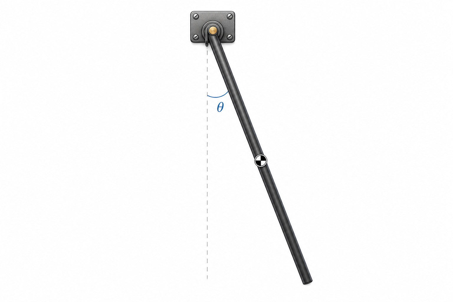
The plant is a uniform rigid rod of length \(\ell\), mass \(m\), and pivot at one end. Its center of mass is at \(\ell / 2\), and its moment of inertia around the pivot is \(I = m\ell^2 / 3\).

The state is the angle \(\theta\) and angular velocity \(\omega\):

\[ \dot{\theta} = \omega, \qquad \dot{\omega} = -\frac{3g}{2\ell}\sin(\theta) - d\omega . \]

There is no input torque in this first example. The only dynamics are gravity and damping. The damping coefficient \(d\) is modeled directly in angular acceleration units.

Define The Plant

First we define the plant node. It is an rg.ODENode, so it has a State namespace and a dstate(...) method. The State namespace stores the physical state. The dstate(...) method returns the right-hand side of the ODE.

class FreePendulum(rg.ODENode):
    class State(rg.NodeState):
        theta: float = rg.var(init=lambda self: cast(FreePendulum, self).theta0)
        omega: float = rg.var(init=lambda self: cast(FreePendulum, self).omega0)

    def dstate(self, state: State) -> State:
        theta_dot = state.omega
        omega_dot = (
            -(3.0 * self.gravity) / (2.0 * self.length) * ca.sin(state.theta)
            - self.damping * state.omega
        )
        return self.State(theta=theta_dot, omega=omega_dot)

The important point is that theta and omega are not method-local variables. They are regelum state variables. Other nodes can connect to FreePendulum.State.theta and FreePendulum.State.omega, and the ODE integrator will update them over time.

Add Observer And Logger

Next we add two ordinary discrete nodes.

Observer reads the plant state and publishes derived signals: \(\sin(\theta)\), \(\cos(\theta)\), and \(\omega\). This is useful because a controller or downstream pipeline often wants angle features rather than the raw angle.

class Observer(rg.Node):
    class Inputs(rg.NodeInputs):
        theta: float = rg.src(FreePendulum.State.theta)
        omega: float = rg.src(FreePendulum.State.omega)

    class State(rg.NodeState):
        sin_angle: float
        cos_angle: float
        angular_velocity: float

    def update(self, inputs: Inputs) -> State:
        return self.State(
            sin_angle=math.sin(inputs.theta),
            cos_angle=math.cos(inputs.theta),
            angular_velocity=inputs.omega,
        )

Logger reads the clock, the plant, and the observer, then appends one sample to its own samples state.

class Logger(rg.Node):
    class Inputs(rg.NodeInputs):
        time: float = rg.src(rg.Clock.time)
        theta: float = rg.src(FreePendulum.State.theta)
        sin_angle: float = rg.src(Observer.State.sin_angle)
        cos_angle: float = rg.src(Observer.State.cos_angle)
        angular_velocity: float = rg.src(Observer.State.angular_velocity)

    class State(rg.NodeState):
        samples: list[tuple[float, float, float, float, float]] = rg.var(init=list)

    def update(self, inputs: Inputs, prev_state: State) -> State:
        sample = (
            inputs.time,
            inputs.theta,
            inputs.sin_angle,
            inputs.cos_angle,
            inputs.angular_velocity,
        )
        prev_state.samples.append(sample)
        return self.State(samples=prev_state.samples)

Here Observer.State.* uses bare annotations intentionally. These variables do not need initial values because Logger reads them only after Observer has produced them in the same observe phase. The annotations still declare state ports, so other nodes can reference Observer.State.sin_angle, Observer.State.cos_angle, and Observer.State.angular_velocity.

Logger.State.samples does need init=list, because the logger receives its previous state as prev_state and mutates the previous sample list with append. The callable list is used instead of [] so every system reset starts from a fresh list object.

Build The System

Now we instantiate the plant and put it into an ODESystem.

pendulum = FreePendulum()
plant = rg.ODESystem(nodes=(pendulum,), dt=BASE_DT)

This line is the bridge between "a node that describes derivatives" and "a phase node that integrates continuous dynamics". Here BASE_DT = "0.01", so the pendulum is integrated on a 10 ms base grid.

Then we instantiate the observer and logger and build the PRS:

observer = Observer()
logger = Logger()

system = rg.PhasedReactiveSystem(
    phases=[
        rg.Phase(
            "plant",
            nodes=(plant,),
            transitions=(rg.Goto("observe"),),
            is_initial=True,
        ),
        rg.Phase(
            "observe",
            nodes=(observer, logger),
            transitions=(rg.Goto(rg.terminate),),
        ),
    ],
    base_dt=BASE_DT,
)

The first phase integrates the continuous plant. The second phase runs the discrete observer and logger. The tick ends at rg.terminate. Вуаля: the system is ready to simulate.

Phase Graph

Every tick starts at init, enters the initial phase, and ends at ⊥.

flowchart LR
    init([init]) --> plant["plant<br/>ODESystem(dt = 0.01)"]
    plant --> observe["observe<br/>Observer + Logger"]
    observe --> done([⊥])

    classDef plant fill:#2f6fed22,stroke:#2f6fed,color:#111318
    classDef observe fill:#15803d22,stroke:#15803d,color:#111318
    class plant plant
    class observe observe

Node Graph

The node graph is the dataflow inside those phases. Solid arrows mean "reads state from another node". Dashed arrows from state show self-reads from the previous tick: FreePendulum reads its own physical state in dstate(...), and Logger reads its own samples tuple before appending a new row. The node colors follow phase colors: blue nodes run in plant, green nodes run in observe.

flowchart LR
    clock["Clock"] --> logger["Logger"]
    pendulum["FreePendulum"] --> observer["Observer"]
    pendulum --> logger
    observer --> logger
    pendulum_state(("state")) -.-> pendulum
    logger_state(("state")) -.-> logger

    classDef plant fill:#2f6fed22,stroke:#2f6fed,color:#111318
    classDef observe fill:#15803d22,stroke:#15803d,color:#111318
    classDef clock fill:transparent,stroke:currentColor,stroke-dasharray:6 4
    classDef state fill:#94a3b822,stroke:#94a3b8,stroke-dasharray:3 3,color:#111318
    class pendulum plant
    class observer,logger observe
    class clock clock
    class pendulum_state,logger_state state

Phase Table

Phase	Nodes	Role
plant	`ODESystem(FreePendulum)`	Integrates the torque-free differential equation.
observe	`Observer`, `Logger`	Publishes observer signals and records samples for plotting.

Node Table

Node	State	Inputs
FreePendulum	`theta`, `omega`	none
Observer	`sin_angle`, `cos_angle`, `angular_velocity`	`FreePendulum.State.theta`, `FreePendulum.State.omega`
Logger	`samples`	`Clock.time`, plant state, observer state

Run The Simulation

The notebook runs the system, reads Logger.State.samples, and plots the observer signals.

system = build_system()
system.run(700)
samples = system.read(Logger.State.samples)

After that we unpack time, sin_angle, cos_angle, and omega, then draw two plots: trigonometric observer outputs on top and angular velocity below. This lets us inspect how the free pendulum swings and damps out over time.

Free pendulum simulation result

Open In Marimo

Open the notebook in molab:

Open in molab

Molab opens the notebook from the published main branch and installs regelum from PyPI, plus plotting dependencies, using the notebook's inline dependency metadata.

Standalone Python listing

from __future__ import annotations

import math
from typing import cast

import casadi as ca

import regelum as rg

BASE_DT = "0.01"
GRAVITY = 9.81
LENGTH = 1.0
DAMPING = 0.08


class FreePendulum(rg.ODENode):
    def __init__(
        self,
        *,
        theta0: float = 0.85,
        omega0: float = 0.0,
        gravity: float = GRAVITY,
        length: float = LENGTH,
        damping: float = DAMPING,
    ) -> None:
        self.theta0 = theta0
        self.omega0 = omega0
        self.gravity = gravity
        self.length = length
        self.damping = damping

    class State(rg.NodeState):
        theta: float = rg.var(init=lambda self: cast(FreePendulum, self).theta0)
        omega: float = rg.var(init=lambda self: cast(FreePendulum, self).omega0)

    def dstate(self, state: State) -> State:  # ty: ignore[invalid-method-override]
        theta_dot = state.omega
        omega_dot = (
            -(3.0 * self.gravity) / (2.0 * self.length) * ca.sin(state.theta)
            - self.damping * state.omega
        )
        return self.State(theta=theta_dot, omega=omega_dot)


class Observer(rg.Node):
    class Inputs(rg.NodeInputs):
        theta: float = rg.src(FreePendulum.State.theta)
        omega: float = rg.src(FreePendulum.State.omega)

    class State(rg.NodeState):
        sin_angle: float
        cos_angle: float
        angular_velocity: float

    def update(self, inputs: Inputs) -> State:
        return self.State(
            sin_angle=math.sin(inputs.theta),
            cos_angle=math.cos(inputs.theta),
            angular_velocity=inputs.omega,
        )


class Logger(rg.Node):
    class Inputs(rg.NodeInputs):
        time: float = rg.src(rg.Clock.time)
        theta: float = rg.src(FreePendulum.State.theta)
        sin_angle: float = rg.src(Observer.State.sin_angle)
        cos_angle: float = rg.src(Observer.State.cos_angle)
        angular_velocity: float = rg.src(Observer.State.angular_velocity)

    class State(rg.NodeState):
        samples: list[tuple[float, float, float, float, float]] = rg.var(init=list)

    def update(self, inputs: Inputs, prev_state: State) -> State:
        sample = (
            inputs.time,
            inputs.theta,
            inputs.sin_angle,
            inputs.cos_angle,
            inputs.angular_velocity,
        )
        prev_state.samples.append(sample)
        return self.State(samples=prev_state.samples)


def build_system() -> rg.PhasedReactiveSystem:
    pendulum = FreePendulum()
    observer = Observer()
    logger = Logger()
    plant = rg.ODESystem(nodes=(pendulum,), dt=BASE_DT)
    return rg.PhasedReactiveSystem(
        phases=[
            rg.Phase(
                "plant",
                nodes=(plant,),
                transitions=(rg.Goto("observe"),),
                is_initial=True,
            ),
            rg.Phase(
                "observe",
                nodes=(observer, logger),
                transitions=(rg.Goto(rg.terminate),),
            ),
        ],
        base_dt=BASE_DT,
    )


def run_response(steps: int = 700) -> list[tuple[float, float, float, float, float]]:
    system = build_system()
    system.run(steps)
    return cast(
        list[tuple[float, float, float, float, float]],
        system.read(Logger.State.samples),
    )


def main() -> None:
    samples = run_response()
    time, theta, sin_angle, cos_angle, omega = samples[-1]
    print(f"time={time:.2f}")
    print(f"theta={theta:.6f}")
    print(f"sin(theta)={sin_angle:.6f}")
    print(f"cos(theta)={cos_angle:.6f}")
    print(f"omega={omega:.6f}")


if __name__ == "__main__":
    main()